Metamaterial Design Through Engineered Environments

Metamaterial design can be viewed as a problem of engineering interactions. Instead of modifying only a material’s intrinsic constituents, we couple a subsystem to an engineered environment. The environment responds to the subsystem and acts back on it, reshaping its effective dynamics.

For wave systems, this perspective connects local resonance, temporal modulation, active feedback, and nonlocal coupling within a common modeling framework. My particular interest is in active implementations, where electronic networks and feedback make these interactions programmable.

The sections below develop this viewpoint through coupled-system equations, local resonance, piezoelectric circuits, and active control.

1. The design principle

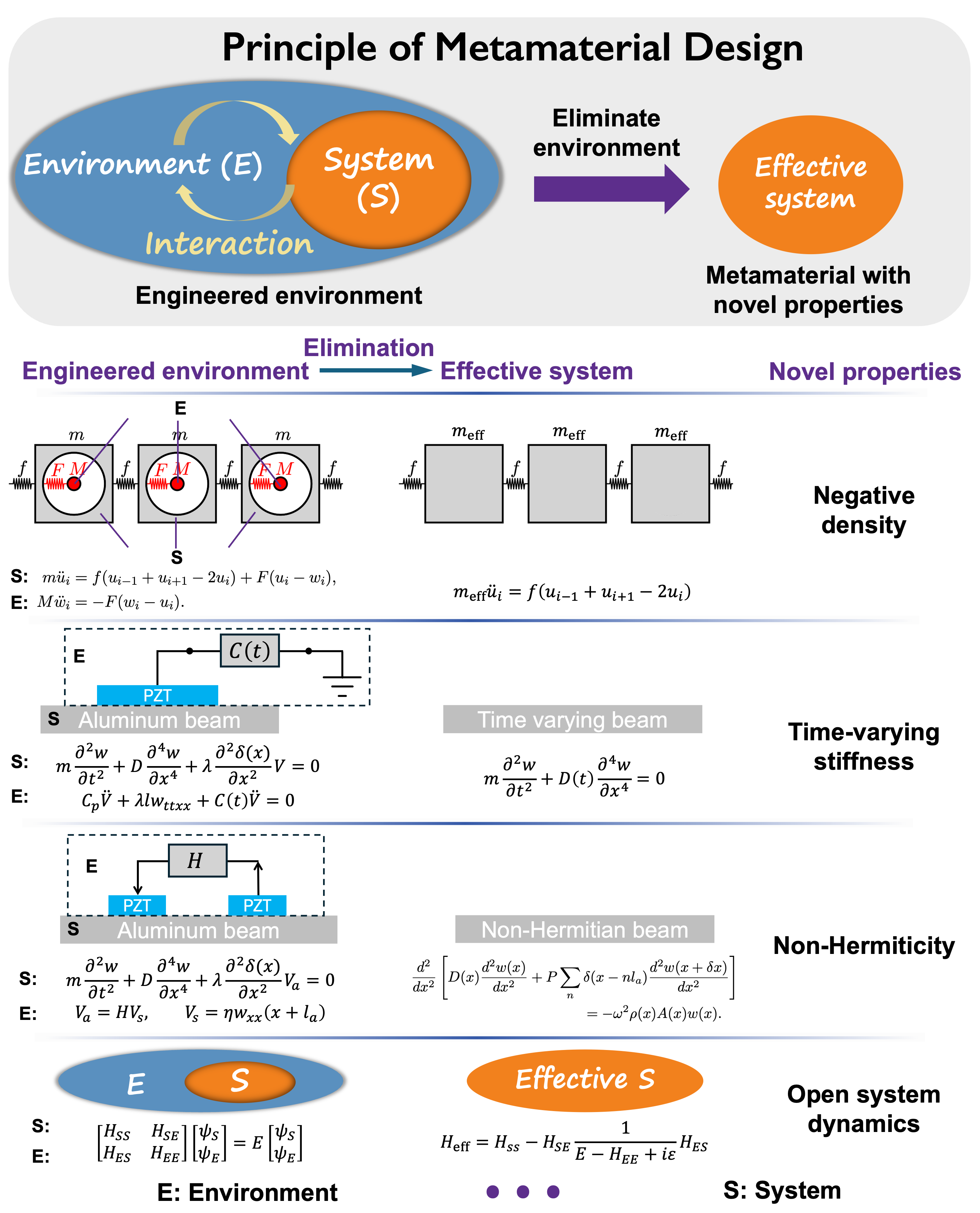
Metamaterial design overview: an engineered environment interacts with a subsystem; eliminating environmental variables produces effective properties, with examples of negative effective mass, time-varying stiffness, non-Hermitian response, and open-system dynamics. — From engineered environments to effective material responses. Click to view the original figure.

We distinguish three ingredients:

Subsystem: the degrees of freedom whose response we want to control, such as the displacement of a beam or a mechanical lattice.
Environment: auxiliary degrees of freedom, such as internal resonators, electrical circuits, controllers, or other coupled modes.
Interaction: the physical or implemented coupling between the two.

The environment need not be spatially outside the subsystem. An internal resonator embedded in a unit cell can play the same mathematical role as a connected electrical network. The partition depends on the response we want to describe.

The design sequence is:

Desired wave response → engineered interactions → effective dynamics → experimental realization.

“Eliminating the environment” means solving for its variables and substituting them into the subsystem equation. The environment remains physically present. Its effects are encoded in an effective operator, which can depend on frequency, position, and time.

2. From coupled equations to an effective system

Consider a linear, time-invariant system in the frequency domain. Let $u$ describe the subsystem and $v$ the environment:

\begin{pmatrix} D_{SS}(\omega) & D_{SE}(\omega) \\ D_{ES}(\omega) & D_{EE}(\omega) \end{pmatrix} \begin{pmatrix}u\\v\end{pmatrix} = \begin{pmatrix}f_S\\f_E\end{pmatrix}.

For a mechanical system, these blocks may come from a dynamic stiffness matrix containing stiffness, inertia, damping, and control terms. When $D_{EE}$ is invertible,

v=D_{EE}^{-1}(f_E-D_{ES}u).

Substitution gives

\underbrace{\left(D_{SS}-D_{SE}D_{EE}^{-1}D_{ES}\right)}_{D_{\mathrm{eff}}(\omega)}u =f_S-D_{SE}D_{EE}^{-1}f_E.

The effective operator is the Schur complement of the environmental block. Its correction contains both the environment’s response and the couplings that connect it to the subsystem. Environmental forcing also changes the effective input; it cannot always be discarded.

Near environmental resonances, the inverse can become large or singular. Damping, boundary conditions, and the chosen frequency range then matter. Eliminating variables is exact where the inverse exists, but replacing the resulting operator with a simple local material parameter generally requires additional approximations.

A corresponding Hamiltonian description

For a block eigenvalue problem $H\psi=z\psi$ , the environmental equation gives

\psi_E=(zI-H_{EE})^{-1}H_{ES}\psi_S,

and therefore

H_{\mathrm{eff}}(z) =H_{SS}+H_{SE}(zI-H_{EE})^{-1}H_{ES}.

The plus sign here and the minus sign in the dynamic-stiffness expression follow from their respective equation conventions. Equivalently,

H_{\mathrm{eff}}(z) =H_{SS}-H_{SE}(H_{EE}-zI)^{-1}H_{ES}.

This resolves a sign ambiguity in the overview figure: a minus sign must be paired with the second resolvent convention. For an outgoing or retarded description, the boundary prescription is commonly written as $z=E+i0^+$ under the corresponding time convention. Finite closed systems, radiation continua, and dissipative environments require different physical interpretations; elimination alone does not imply loss or non-Hermiticity.

3. Local resonance and effective inertia

Take a one-dimensional chain of outer masses $m$ coupled by springs of stiffness $k$ . Each cell contains an internal mass $M$ connected to the outer mass by a spring of stiffness $\kappa$ . Let $u_n$ and $v_n$ be the outer and inner displacements:

m\ddot u_n =k(u_{n-1}+u_{n+1}-2u_n)+\kappa(v_n-u_n),

M\ddot v_n=-\kappa(v_n-u_n).

With harmonic motion proportional to $e^{-i\omega t}$ ,

v_n=\frac{\kappa}{\kappa-M\omega^2}u_n.

Eliminating $v_n$ yields

-\omega^2m_{\mathrm{eff}}(\omega)u_n =k(u_{n-1}+u_{n+1}-2u_n),

where

m_{\mathrm{eff}}(\omega) =m+\frac{\kappa M}{\kappa-M\omega^2} =m+\frac{M\omega_0^2}{\omega_0^2-\omega^2}, \qquad \omega_0^2=\frac{\kappa}{M}.

In this ideal undamped model, the effective mass is negative for

\omega_0<\omega<\omega_0\sqrt{1+M/m}.

This is a dynamic response, not a negative constituent mass. At low frequency the internal mass follows the outer mass and $m_{\mathrm{eff}}\to m+M$ . Near resonance their relative motion strongly changes the force–acceleration relation. Damping regularizes the resonance and generally makes the effective mass complex. Converting a cell-level effective mass into a continuum density also requires an appropriate homogenization regime.

4. Electrical environments and time-varying stiffness

A piezoelectric patch couples mechanical deformation to electrical variables. Connecting it to a circuit changes the electrical boundary condition, which acts back on the mechanical structure.

For example, after a suitable reduction and homogenization, a flexural beam may be modeled by

\mu\,\partial_t^2w +\partial_x^2\!\left[D_{\mathrm{eff}}(x,t)\,\partial_x^2w\right]=0,

where $\mu$ is mass per unit length and $D_{\mathrm{eff}}$ is an effective bending rigidity. If the rigidity is spatially uniform, the second term reduces to $D_{\mathrm{eff}}(t)\partial_x^4w$ .

Here the circuit is the engineered environment. A programmed change in its response can produce a temporal change in effective rigidity. The microscopic beam need not physically change its geometry during the modulation.

In our work on temporal refraction and reflection in elastic beams, piezoelectric patches and electronic circuitry create time-dependent effective elastic properties. This enables temporal scattering and control of wave amplitude and frequency.

The local coefficient $D_{\mathrm{eff}}(t)$ is a reduced model. An electrical environment with significant internal dynamics can instead generate memory:

M(x,t)=\int_{-\infty}^{t} \mathcal D(x;t,t')\,\partial_x^2w(x,t')\,dt'.

Here $M$ denotes bending moment, not the internal resonator mass used above. A frequency-dependent circuit cannot in general be replaced by an instantaneous stiffness, especially during rapid modulation. Full coupled dynamics should be retained when the reduced approximation fails.

5. Active feedback as an interaction-design tool

An active implementation separates sensing, signal processing, and actuation. In a time-invariant frequency-domain model, write

y=C(\omega)u,\qquad f_a=B(\omega)G(\omega)y.

Here $C$ maps motion to a sensed signal, $G$ is the controller, and $B$ maps the controller output to an applied force. If $D_0u=f_{\mathrm{ext}}+f_a$ , then

\left[D_0(\omega)-B(\omega)G(\omega)C(\omega)\right]u =f_{\mathrm{ext}}.

The controller therefore contributes a designed correction to the dynamic operator. Its sign depends on the implemented feedback convention.

This suggests several routes:

Local feedback can modify apparent stiffness, damping, or inertia over a chosen band.
Sensing at one location and actuating at another creates nonlocal interactions.
Independently designed directional channels can enable nonreciprocal coupling; activity alone does not guarantee nonreciprocity.
Gain, loss, and suitable asymmetric couplings can produce non-Hermitian effective dynamics. Not every active controller does so.
Time-dependent control requires a time-domain or frequency-mixing description rather than a single-frequency transfer function.

The value of active control is not unlimited freedom: it is a wider, programmable interaction space, constrained by causality, bandwidth, delay, noise, actuator limits, and closed-loop stability.

6. Designing backward from the desired waves

A practical workflow starts with an observable target rather than a material label:

Specify the response. Choose the desired transmission, reflection, frequency conversion, localization, or amplification, including the operating band.
Identify the effective operator. Determine which terms or couplings could produce that response.
Choose the environment. Select resonators, circuits, controllers, or auxiliary modes that can implement the required correction.
Design the interactions. Set sensing and actuation locations, coupling strengths, transfer functions, and modulation protocols.
Check the reduction. Compare effective predictions against the full coupled model, including dispersion and memory where relevant.
Validate the realization. Test stability, robustness, finite-size effects, and measured wave fields, not just fitted parameter values.

The input and output waves in the homepage diagram are a conceptual illustration. A real experiment may involve reflection, several transmitted channels, sidebands, and energy exchange with a controller. A complete description must include the relevant channels.

This perspective treats metamaterials as physical systems whose effective dynamics are designed through their interactions. Active environments make those interactions tunable, connecting a general design principle to realizable control of waves.